The following article introduces how database queries are formed and executed, and how popular databases behave differently in optimization scenarios, due to how queries are formed in their engines.
https://buttondown.email/jaffray/archive/the-case-of-a-curious-sql-query/
Languages that suffer success often have to do so by selling out and adding features that go against some of the original purposes of their design.
SQL is a great example of a language built on very solid foundations: it comes from the idea that we should define an algebra for data retrieval, and then we can formally define how that algebra should behave, and then we can have a common tongue between humans who want to query databases and databases who want to execute CPU instructions.
This is the kind of thing that excites people who implement query engines and are conflict averse because it creates an authoritative source for how queries should behave. We’ve formally defined what it means for this given operator to run, so if there’s any dispute, we have the technology to figure out what the result “should be.”
This is particularly nice in the presence of optimizing such queries. For example, “predicate pushdown” is a well-known optimization which says that if I have a predicate on an inner join that only references columns from one of its arms, I can push it down into one of those arms and reduce the size of the data I have to join:
SELECT * FROM abc INNER JOIN def ON abc.a = def.d AND abc.b = 4
can become
SELECT * FROM (SELECT * FROM abc WHERE abc.b = 4) INNER JOIN def ON abc.a = def.d
Which may or may not be hard to convince yourself of, but if you have formal definitions of what a join is laid out in front of you, it becomes very obvious that this is correct.
Things like this got messier when people actually started using these languages and started caring about properties (say, the order of a result set) of a relational query that the original model didn’t have a notion of. Of course, that one is fairly easily resolved, but it is sometimes more difficult, and we get back into the realm of ambiguity.
Here is my favourite SQL query:
SELECT count(*) FROM one_thousand INNER JOIN one_thousand ON random() < 0.5
Where one_thousand is a single column table of the numbers 0, 1, … 999.
What number do we expect to see from this query? To me, intuitively, it seems like we should be evaluating this predicate on each pair of rows from the two inputs, so we’d expect to get about half of them, so we should see about ~500000 rows. And if we run this in DuckDB, that’s indeed more or less what we see:
D SELECT count(*) FROM one_thousand a INNER JOIN one_thousand b ON random() < 0.5;
┌──────────────┐
│ count_star() │
├──────────────┤
│ 499910       │
└──────────────┘
D SELECT count(*) FROM one_thousand a INNER JOIN one_thousand b ON random() < 0.5;
┌──────────────┐
│ count_star() │
├──────────────┤
│ 499739       │
└──────────────┘
D SELECT count(*) FROM one_thousand a INNER JOIN one_thousand b ON random() < 0.5;
┌──────────────┐
│ count_star() │
├──────────────┤
│ 500054       │
└──────────────┘
D
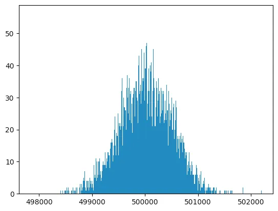
I ran this query 1000 times, and the mean result was 500011.6034, hovering right around the expected mean of 500000.
We should expect these results to be binomially distributed, and if we plot a histogram of a bunch of runs, that’s basically what we see:
Let’s try a different database, SQLite. In SQLite, random() returns a 64-bit signed integer so this query is slightly different, but just for consistency I’m going to write it the same way:
sqlite> select count(*) from one_thousand a inner join one_thousand b on random() < 0.5;
511000
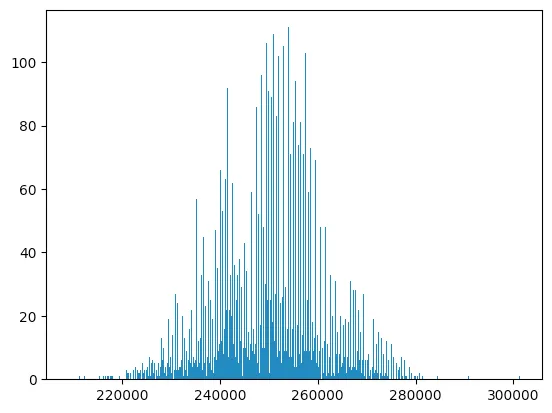
Looks pretty reasonable. Doing another 10000 trials, we get a mean of 499865.8, which seems like we’re getting the same behaviour as DuckDB. Now let’s plot those 10000 trials in a histogram:

Hm! Looks suspiciously different than DuckDB! Not only are the points much more sparse, the variance of the distribution is also much higher. What’s going on here? SQLite plans are unfortunately not the most enlightening:
sqlite> explain select count(*) from one_thousand a inner join one_thousand b on random() < 0.5;
addr  opcode         p1    p2    p3    p4             p5  comment
----  -------------  ----  ----  ----  -------------  --  -------------
0     Init           0     17    0                    0   Start at 17
1     Null           0     1     1                    0   r[1..1]=NULL
2     OpenRead       0     2     0     0              0   root=2 iDb=0; one_thousand
3     OpenRead       1     2     0     0              0   root=2 iDb=0; one_thousand
4     Explain        4     0     0     SCAN a         0
5     Rewind         0     13    0                    0
6       Function       0     0     2     random(0)      0   r[2]=func()
7       Ge             3     12    2                    80  if r[2]>=r[3] goto 12
8       Explain        8     0     0     SCAN b         0
9       Rewind         1     13    0                    0
10        AggStep        0     0     1     count(0)       0   accum=r[1] step(r[0])
11      Next           1     10    0                    1
12    Next           0     6     0                    1
13    AggFinal       1     0     0     count(0)       0   accum=r[1] N=0
14    Copy           1     4     0                    0   r[4]=r[1]
15    ResultRow      4     1     0                    0   output=r[4]
16    Halt           0     0     0                    0
17    Transaction    0     0     1     0              1   usesStmtJournal=0
18    Real           0     3     0     0.5            0   r[3]=0.5
19    Goto           0     1     0                    0
But what’s going on here becomes a bit more obvious if we look at a few more sample results of our query:
sqlite> select count(*) from one_thousand a inner join one_thousand b on random() < 0.5;
481000
sqlite> select count(*) from one_thousand a inner join one_thousand b on random() < 0.5;
486000
sqlite> select count(*) from one_thousand a inner join one_thousand b on random() < 0.5;
503000
sqlite> select count(*) from one_thousand a inner join one_thousand b on random() < 0.5;
518000
They’re notably all divisible by 1000. Recall the query transformation we opened with:
SELECT * FROM abc INNER JOIN def ON abc.a = def.d AND abc.b = 4
=>
SELECT * FROM (SELECT * FROM abc WHERE abc.b = 4) INNER JOIN def ON abc.a = def.d
This optimization is valid because abc.b = 4 doesn’t use any of the columns from def, so we can push it down and evaluate it directly on abc.
In this query:
select count(*) from one_thousand a inner join one_thousand b on random() < 0.5;
random() < 0.5 doesn’t depend on any columns in one_thousand, and so SQLite concludes that it’s valid to transform the query to something like:
SELECT count(*) FROM
  (SELECT * FROM one_thousand WHERE random() < 0.5)
    INNER JOIN
  one_thousand
    ON true;
Which, since the right side of this join has exactly 1000 rows, will always result in a number divisible by 1000.
For a final example, let’s look at CockroachDB (disclosure, disclosure, former employer, used to work on the query optimizer specifically).
Doing 10000 trials of our query in CockroachDB, we get a mean of 249889.969(!) and the following distribution:
You might be able to guess what’s going on here. Here’s an EXPLAIN plan for the query:
                              info
----------------------------------------------------------------
 • group (scalar)
 └── • cross join
     ├── • filter
     │   │ filter: random() < 0.5
     │   └── • scan
     └── • filter
         │ filter: random() < 0.5
         └── • scan
Aha! CockroachDB notes that random() < 0.5 isn’t bound by either side of the join, and so we can push it down into both sides. Now we are effectively performing this filter twice for each eventual output row, and thus we end up with about 25% of the rows in the final output. You’ll also notice it’s much spikier than the other ones, with more outliers, I suppose this is partly because this execution plan means we are more likely to output numbers which are more composite than ones which are closer to being prime.
As one last example, in some SQL dialects there is a “set returning function” called generate_series which can be used to construct tables like one_thousand. In CockroachDB:
defaultdb=> select * from generate_series(0, 999);
 generate_series
-----------------
               0
               1
               2
             ...
             999
We can again construct our query but using this function instead of a reference to an explicit table:
select count(*) from
  generate_series(0,999) a
    inner join
  generate_series(0,999)
    on random() < 0.5
Running 10000 trials of this, I got a mean of 241700.0. Surprisingly far from the expected mean! Plotting the histogram shows us why:
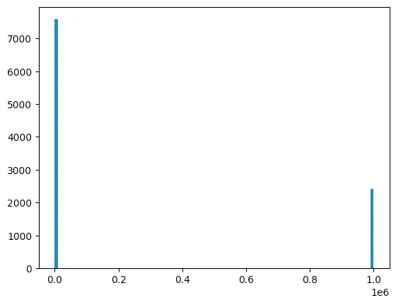
~75% of the results were 0, and ~25% were 1000000. To see why, we can look at the EXPLAIN:
                 info
---------------------------------------
 • group (scalar)
 └── • cross join
     ├── • cross join
     │   ├── • project set
     │   │   └── • emptyrow
     │   └── • filter: random() < 0.5
     │       └── • emptyrow
     └── • cross join
         ├── • project set
         │   └── • emptyrow
         └── • filter: random() < 0.5
             └── • emptyrow
For reasons that aren’t apparent in this simple example, these generate_series get planned as joins against some input. In this case, the input is just the unit row (zero columns, one row) named “emptyrow” in this plan.
For our query, the random() < 0.5 filter gets pushed down both sides all the way to this unit row. Where on any execution, it either gets filtered or not. So if you win both coin flips, you get the full output, otherwise, you get nothing.
Is any of this a particularly important consideration? Eh. No. I dunno. Not really. I don’t think you could make a particularly compelling claim that any of these behaviours are wrong. I don’t know what, if anything, the SQL spec has to say on this, but I think the industry generally seems to agree that’s more of a gentle suggestion than anything resembling a “standard.”
This kind of thing (impure functions in a declarative language, specifically) does cause actual problems in other contexts, which we will talk about someday, but for now I think it’s a fun little mind bender that gives you some insight into the internals of these databases query engines without having to actually look at any code.
#reads #justin jaffray #sql #optimization #internals #sqlite #cockroachdb #duckdb